Packages

library(caret)

Loading required package: ggplot2

Loading required package: lattice

library(glmnet)

Loading required package: Matrix

Loaded glmnet 4.1-8

library(purrr)


Attaching package: 'purrr'

The following object is masked from 'package:caret':

    lift

Functions

get_rmse <- function(errors){
  sqrt(mean(errors^2))
}

LOO-CV

Custom LOO-CV function

This function implement a not elegant function for testing the loo-cv. Is useful for understanding the idea:

my_loocv <- function(fit){
  
  dat <- fit$model
  y <- all.vars(fit$call)[1]
  
  errors <- vector(mode = "numeric", length = nrow(dat))
  
  for(i in 1:nrow(dat)){
    to_pred_i <- dat[i, ]
    fit_no_i <- update(fit, data = dat[-i, ])
    pred_i <- predict(fit_no_i, to_pred_i)
    errors[i] <- pred_i - to_pred_i[1, y]
  }
  return(errors)
}

Comparing with the function from caret, this is the OLS model:

caret_ols <- train(mpg ~ disp + wt, 
               data = mtcars, 
               trControl=trainControl(method="LOOCV"), 
               method="lm")

My custom function:

standard_ols <- lm(mpg ~ disp + wt, data = mtcars)
my_loocv <- get_rmse(my_loocv(standard_ols))

The output is exactly the same:

caret_ols$results["RMSE"] == my_loocv

  RMSE
1 TRUE

LOO-CV and model complexity

predictors <- colnames(mtcars) # getting all predictors
predictors <- predictors[-(predictors == "mpg")] # keeping only Xs

fit_list <- vector(mode = "list", length = length(predictors))

fit_i <- lm(mpg ~ 1, data = mtcars)

for(i in 1:length(predictors)){
  fit_i <- update(fit_i, formula(paste(". ~ . +", predictors[i])))
  fit_list[[i]] <- fit_i
}

Computing the actual LOO-CV:

my_loocv <- function(fit){
  
  dat <- fit$model
  y <- all.vars(fit$call)[1]
  
  errors <- vector(mode = "numeric", length = nrow(dat))
  
  for(i in 1:nrow(dat)){
    to_pred_i <- dat[i, ]
    fit_no_i <- update(fit, data = dat[-i, ])
    pred_i <- predict(fit_no_i, to_pred_i)
    errors[i] <- pred_i - to_pred_i[1, y]
  }
  return(errors)
}

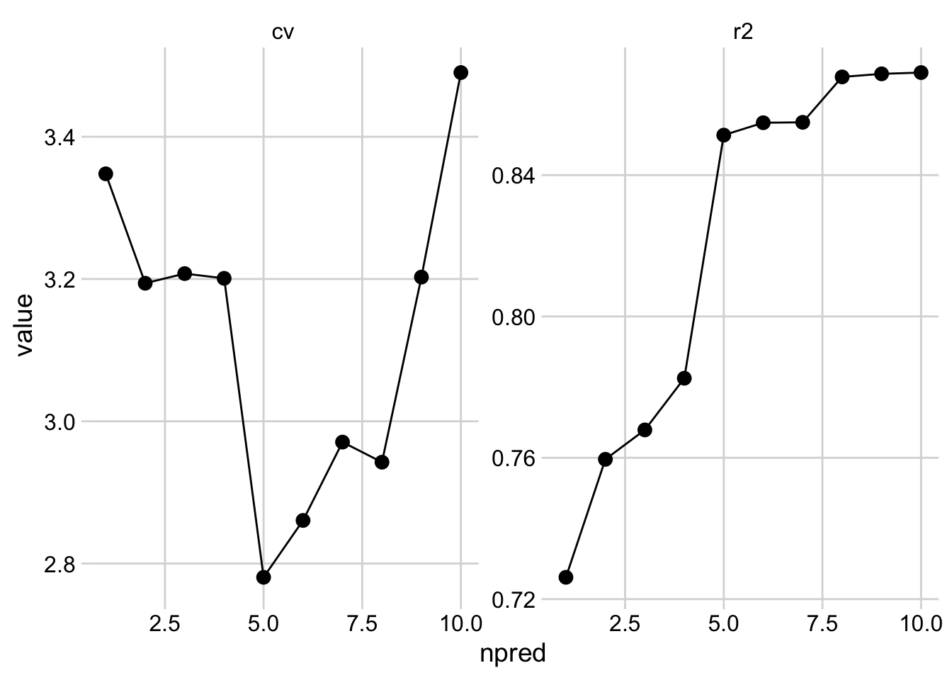
cv <- map_dbl(fit_list, function(x) get_rmse(my_loocv(x))) # get loo-cv mean error
npred <- map_dbl(fit_list, function(i) length(all.vars(i$call))-2) # get number of predictors
r2 <- map_dbl(fit_list, function(mod) summary(mod)$r.squared) # get rsquared from fitted models

loo_cv <- data.frame(
  cv, r2, npred
)

# Plotting

loo_cv %>% 
  tidyr::pivot_longer(c(1,2), names_to = "measure", values_to = "value") %>% 
  ggplot(aes(x = npred, y = value)) +
  geom_line() +
  geom_point(size = 3) +
  facet_wrap(~measure, scales = "free") +
  cowplot::theme_minimal_grid()

LOO-CV and Lasso regression

grid <- 10^seq(1, -2, length = 100) # grid of lambda values
x <- model.matrix(mpg ~ ., mtcars)[, -1] # predictors
y <- mtcars$mpg # response variable

Fitting the lasso regression:

fit_lasso <- glmnet(x, y, alpha = 1, lambda = grid)

Custom function for computing the lasso and loo-cv:

my_loocv_lasso <- function(dat, fit){
  
  errors <- vector(mode = "list", length = nrow(dat))
  
  for(i in 1:nrow(dat)){
    to_pred_i <- x[i, ]
    fit_no_i <- glmnet(x[-i, ], y[-i], alpha = 1, lambda = grid)
    pred_i <- predict(fit_no_i, newx = t(to_pred_i))
    errors[[i]] <- pred_i - y[i]
  }
  return(errors)
} 

get_min <- function(target, to_minimize){
  target[which.min(to_minimize)]
}

Computing the loo-cv:

errors_lasso <- my_loocv_lasso(mtcars, fit_lasso) # loo-cv

cv_lasso <- do.call(rbind, errors_lasso) # combining lists

mse_lasso <- apply(cv_lasso, 2, function(x) mean(x^2)) # computing error

Plotting the \(\lambda\) value as a function of the mean-squared error:

plot(grid, mse_lasso)

The minimum error is associated with the 0.7564633.