# Packages

library(tidyverse)
library(pwr)
library(BayesFactor)

# Seed for simulation

set.seed(2021)
General idea
The sensitivity analysis is a way to estimate the effect size that a given experiment can reach with a certain sample size, desired power and alpha level [@perugini2018practical].
The power analysis is usually considered a procedure that estimate a single number (i.e., the sample size) required for a given statistical analysis to reach a certain power level. Is better to consider the power level as a function with fixed and free parameters.
In the case of the a priori power analysis, we fix the power level (e.g., \(1 - \beta = 0.80\)) the alpha level (e.g., \(\alpha = 0.05\)“) and the hypothetical effect size (e.g, \(d = 0.3\)). Then we simulate or derive analytically the minimum sample size required for reaching the target power level, given the effect size.
A more appropriate approach is to consider the sample size a free parameter and calculate the power level for a range of sample size, obtaining the power curve. This is very easy using the pwr package. We assume:
- \(1-\beta = 0.8\)
- \(\alpha = 0.05\)
- \(d = 0.3\)
- an independent sample t-test situation
power_analysis <- pwr::pwr.t.test(
  d = 0.3,
  power = 0.8,
  sig.level = 0.05
)
power_analysis
     Two-sample t test power calculation

              n = 175.3847
              d = 0.3
      sig.level = 0.05
          power = 0.8
    alternative = two.sided

NOTE: n is number in *each* group
From the output we need 175.3846666 subjects per group for reaching the desired power level. As said before a better approach is analyzing the entire power curve. We can simply plot the power_analysis object:
plot(power_analysis)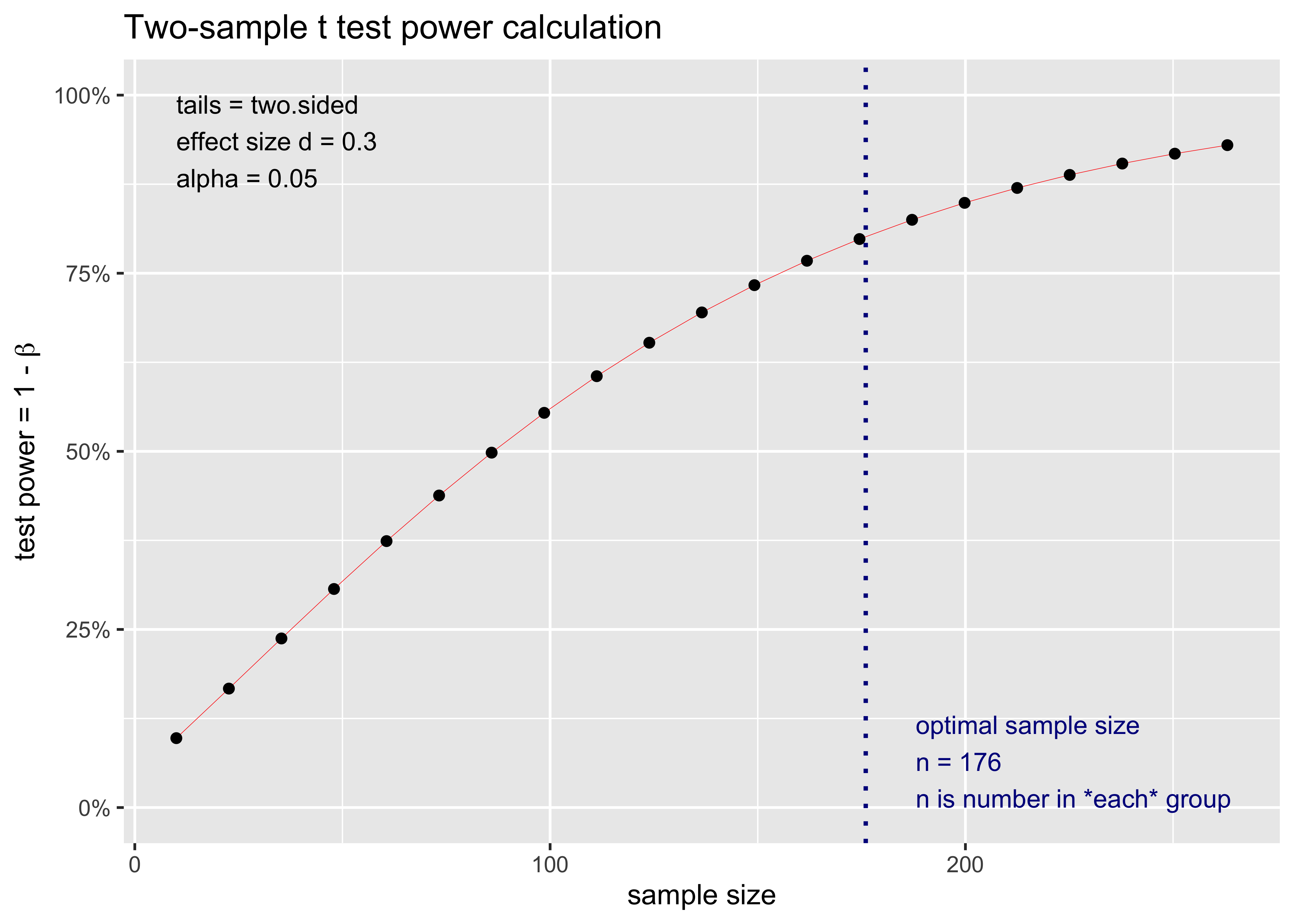
Power by simulation
The previous example is based on the analytically power computation that is possible for simple statistical test. A more general approach is the power analysis by simulation.
If we know the statistical assumptions of our analysis we can simulate data accordingly several times (e.g., 10000 simulations) and simply count the number of p values below the alpha level. This is a little bit too much for a simple t-test but can be really insightful.
We need to simulate two groups sampled from two populations with different mean (our effect size) and with the same standard deviation. We can simulate directly on the cohen's d scale setting the standard deviation to 1 and the mean difference to the desired d level.
For obtaining the power curve we need a range of sample size from 10 to 200 for example.
There are multiple ways to approach a simulation. Here I declare my parameters and create a grid of values using the tidyr::expand_grid() function to create all combinations. The I simply need to loop for each row, generate data using rnorm, calculate the t-test and then count how many p-values are below the alpha level.
mp0 <- 0
mp1 <- 0.3
sd_p <- 1
# d = mp1 - mp0 / sigma = (0.3 - 0) / 1 = 0.3
sample_size <- seq(10, 200, 30)
nsim <- 1000
alpha_level <- 0.05

sim <- expand_grid(
  mp0,
  mp1,
  sd_p,
  sample_size,
  nsim = 1:nsim,
  p_value = 0
)

# Using the for approach for clarity, *apply or map is better

for(i in 1:nrow(sim)){
  g0 <- rnorm(sim$sample_size[i], sim$mp0[i], sim$sd_p[i])
  g1 <- rnorm(sim$sample_size[i], sim$mp1[i], sim$sd_p[i])
  sim[i, "p_value"] <- t.test(g0, g1)$p.value
}

sim %>%
  group_by(sample_size, mp1) %>%
  summarise(power = mean(p_value < alpha_level)) %>%
  ggplot(aes(x = sample_size, y = power)) +
  geom_point(size = 3) +
  geom_line() +
  ggtitle(paste("Effect size = ", sim$mp1[1]))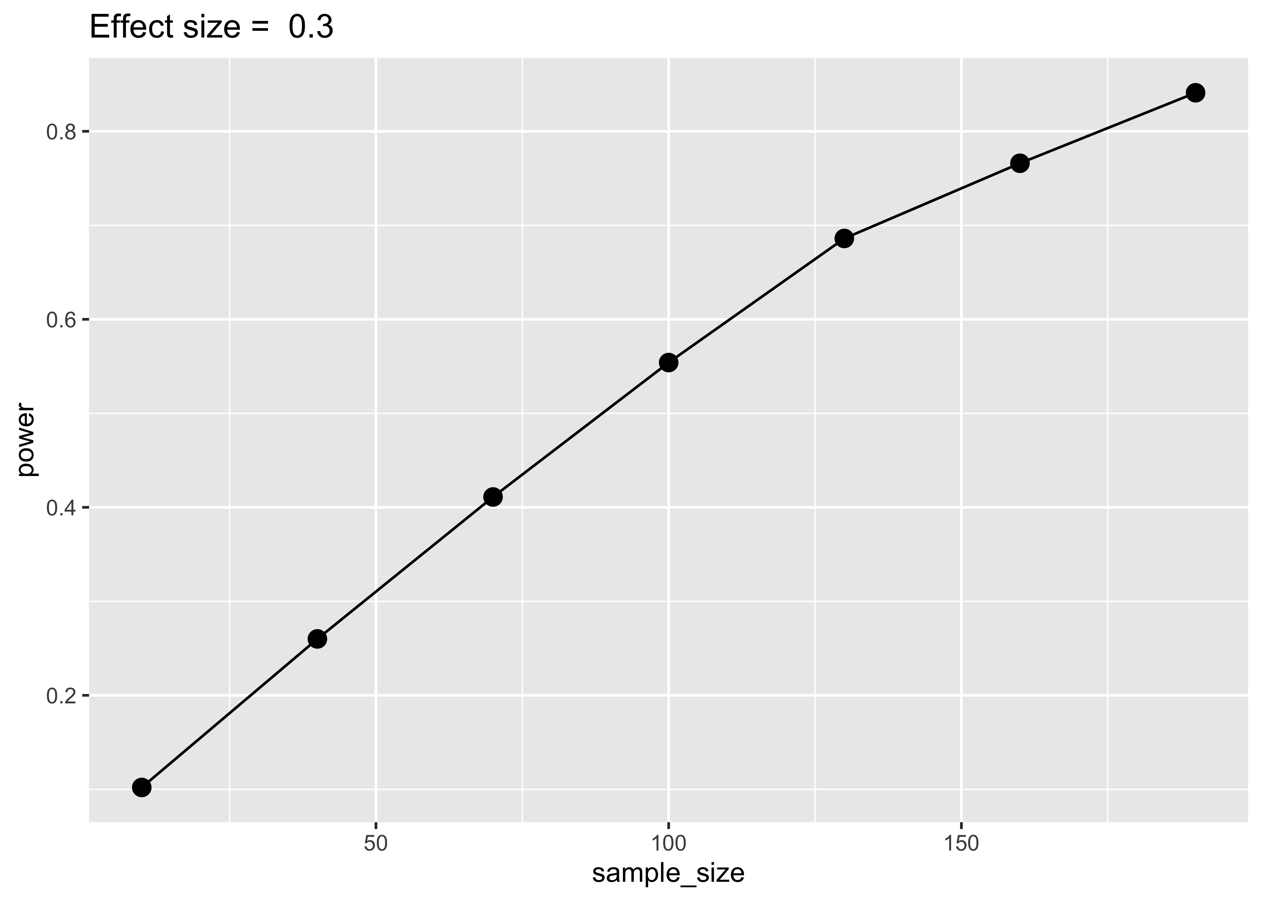
The result is very similar to the pwr result. Increasing the number of simulation will stabilize the results. As said before, using this approach for a t-test is not convenient but with the same code and idea we can simulate an unequal variance situation or having different sample size per group.
Sensitivity Analysis
Using the same approach as before, we can perform a sensivity analysis simply changing our free parameters in the previous simulation. The sensitivity analysis is usually performed with a given sample size and the the free parameter will be the effect size. We can use a range from 0 (the null effect) to 1 and fixing a sample size of 50 subjects per group.
mp0 <- 0
mp1 <- seq(0, 1, 0.2)
sd_p <- 1
sample_size <- 50
nsim <- 1000
alpha_level <- 0.05

sim <- expand_grid(
  mp0,
  mp1,
  sd_p,
  sample_size,
  nsim = 1:nsim,
  p_value = 0
)

# Using the for approach for clarity, *apply or map is better

for(i in 1:nrow(sim)){
  g0 <- rnorm(sim$sample_size[i], sim$mp0[i], sim$sd_p[i])
  g1 <- rnorm(sim$sample_size[i], sim$mp1[i], sim$sd_p[i])
  sim[i, "p_value"] <- t.test(g0, g1)$p.value
}

sim %>%
  group_by(mp1, sample_size) %>%
  summarise(power = mean(p_value < alpha_level)) %>%
  ggplot(aes(x = mp1, y = power)) +
  geom_point(size = 3) +
  geom_line() +
  geom_hline(yintercept = 0.8, linetype = "dashed", size = 1, col = "red") +
  ggtitle(paste("Sample size = ", sim$sample_size[1]))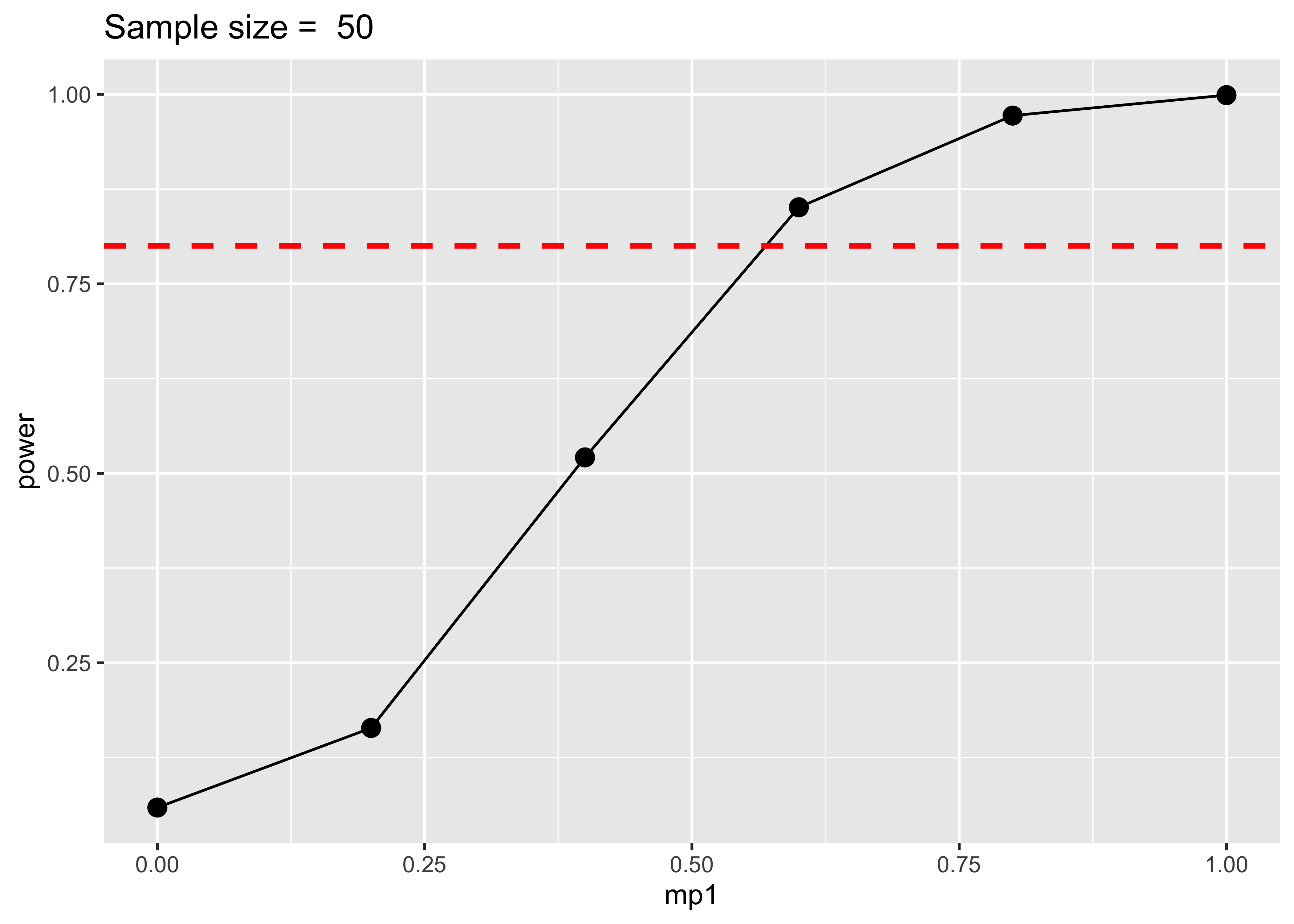
With the simulation approach we simply have to change our grid of values and calculate the power grouping for effect size instead of sample size. Here we understand that with a sample size of 50 we can detect with 80% power an effect size of ~0.6. If the true effect size is lower than the maximum detectable effect size, we are using an under-powered design.
Script
## -----------------------------------------------------------------------------
## Script: Sensitivity analysis
##
## Author: Filippo Gambarota
## -----------------------------------------------------------------------------

# Packages ----------------------------------------------------------------

library(tidyverse)
library(furrr)

# Environment -------------------------------------------------------------

set.seed(2021)

# Functions ---------------------------------------------------------------

# Find the closest target from a vector

find_closest_n <- function(vector, target){
  index <- which.min(abs(vector - target))
  out <- vector[index]
  return(out)
}

# Return the minimun effect size given a sample size and the power level

min_effect <- function(data, sample_size, power_level){
  ns <- find_closest_n(unique(data$sample_size), sample_size)
  min(data$effect_size[data$sample_size == ns & data$power >= power_level])
}

# Calculate power

compute_power <- function(data, alpha){
  data %>%
    group_by(sample_size, effect_size) %>%
    summarise(power = mean(ifelse(p_value < alpha, 1, 0)))
}

# Plot the contour

power_contour <- function(data){
  data %>%
    ggplot(aes(x = sample_size, y = effect_size, z = power)) +
    geom_contour_filled(breaks = seq(0,1,0.1)) +
    coord_cartesian() +
    cowplot::theme_minimal_grid()
}

# Plot the power curve

power_curve <- function(data, n){
  ns <- find_closest_n(unique(data$sample_size), n)
  data %>%
    filter(sample_size == ns) %>%
    ggplot(aes(x = effect_size, y = power)) +
    geom_point() +
    geom_line() +
    cowplot::theme_minimal_grid() +
    ggtitle(paste("Sample size =", ns))
}

# Setup simulation --------------------------------------------------------

sample_size <- seq(10, 500, 50)
effect_size <- seq(0, 1, 0.1)
nsim <- 1000

sim <- expand_grid(
  sample_size,
  effect_size,
  sim = 1:nsim
)

# Test --------------------------------------------------------------------

plan(multisession(workers = 4))

sim$p_value <- furrr::future_map2_dbl(sim$sample_size, sim$effect_size, function(x, y){
  g0 <- rnorm(x, 0, 1)
  g1 <- rnorm(x, y, 1)
  t.test(g0, g1)$p.value
}, .options = furrr_options(seed = TRUE))

# Computing power

sim_power <- compute_power(sim, alpha = 0.05)

# Plots -------------------------------------------------------------------

# Contour plot

power_contour(sim_power)

# Power curve

power_curve(sim_power, 200)
Bayesian
sim <- expand_grid(
  mp0,
  mp1,
  sd_p,
  sample_size,
  nsim = 1:nsim,
  p_value = 0,
  bf = 0
)

# Using the for approach for clarity, *apply or map is better

for(i in 1:nrow(sim)){
  g0 <- rnorm(sim$sample_size[i], sim$mp0[i], sim$sd_p[i])
  g1 <- rnorm(sim$sample_size[i], sim$mp1[i], sim$sd_p[i])
  sim[i, "p_value"] <- t.test(g0, g1)$p.value
  sim[i, "bf"] <- extractBF(ttestBF(g0,g1))$bf
}

sim %>%
  group_by(mp1, sample_size) %>%
  summarise(power = mean(p_value < alpha_level),
            bf = mean(log(bf))) %>%
  pivot_longer(c(power, bf), names_to = "metric", values_to = ".value") %>%
  ggplot(aes(x = mp1, y = .value)) +
  facet_wrap(~metric, scales = "free") +
  geom_point(size = 3) +
  geom_line() +
  ggtitle(paste("Sample size = ", sim$sample_size[1]))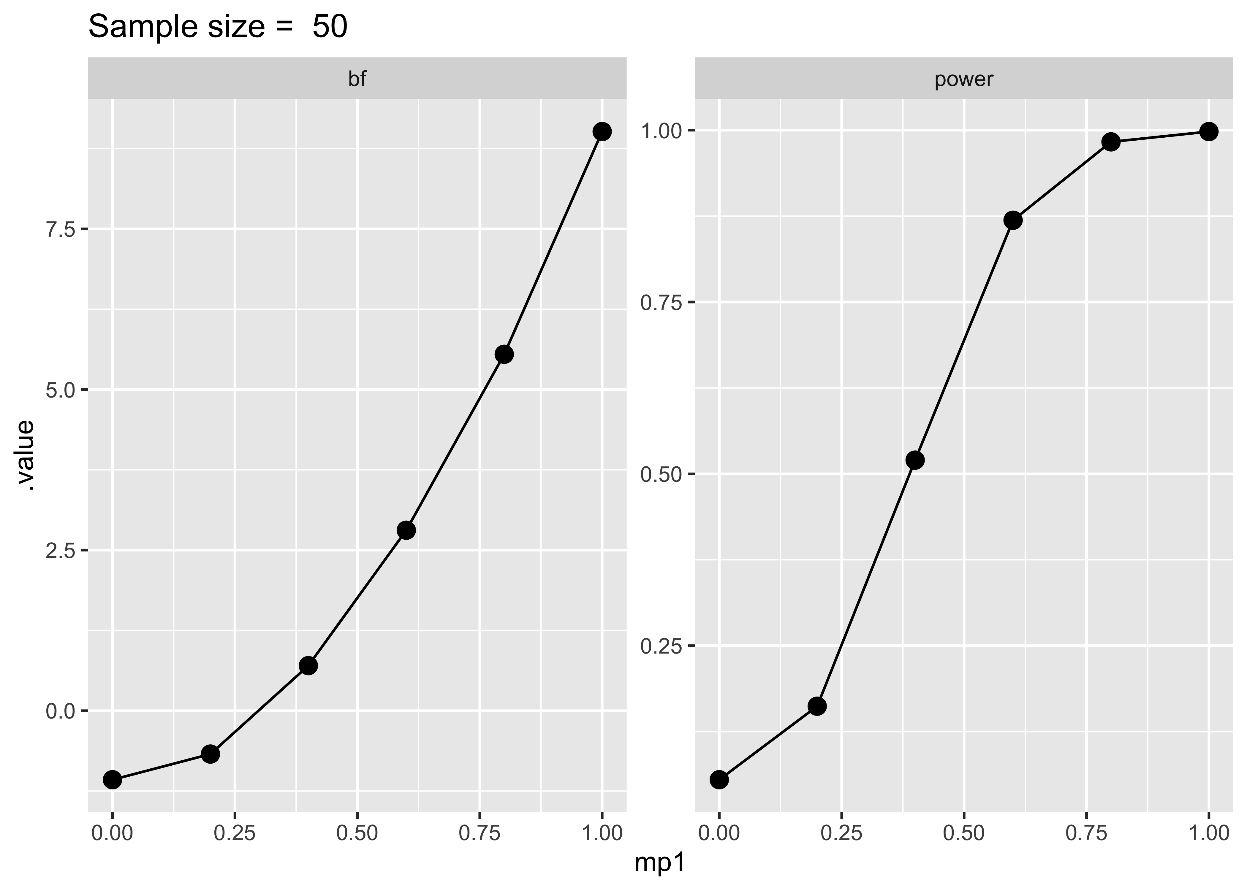
Session info
sessionInfo()R version 4.2.3 (2023-03-15)
Platform: aarch64-apple-darwin20 (64-bit)
Running under: macOS 14.4.1
Matrix products: default
BLAS: /Library/Frameworks/R.framework/Versions/4.2-arm64/Resources/lib/libRblas.0.dylib
LAPACK: /Library/Frameworks/R.framework/Versions/4.2-arm64/Resources/lib/libRlapack.dylib
locale:
[1] en_US.UTF-8/en_US.UTF-8/en_US.UTF-8/C/en_US.UTF-8/en_US.UTF-8
attached base packages:
[1] stats graphics grDevices utils datasets methods base
other attached packages:
[1] BayesFactor_0.9.12-4.7 Matrix_1.5-3 coda_0.19-4
[4] pwr_1.3-0 lubridate_1.9.2 forcats_1.0.0
[7] stringr_1.5.0 dplyr_1.1.2 purrr_1.0.1
[10] readr_2.1.4 tidyr_1.3.0 tibble_3.2.1
[13] ggplot2_3.5.0 tidyverse_2.0.0
loaded via a namespace (and not attached):
[1] Rcpp_1.0.10 compiler_4.2.3 pillar_1.9.0 tools_4.2.3
[5] digest_0.6.31 lattice_0.20-45 timechange_0.2.0 jsonlite_1.8.4
[9] evaluate_0.20 lifecycle_1.0.3 gtable_0.3.3 pkgconfig_2.0.3
[13] rlang_1.1.0 cli_3.6.1 rstudioapi_0.14 parallel_4.2.3
[17] yaml_2.3.7 mvtnorm_1.1-3 xfun_0.39 fastmap_1.1.1
[21] withr_2.5.0 knitr_1.42 MatrixModels_0.5-1 generics_0.1.3
[25] vctrs_0.6.2 htmlwidgets_1.6.2 hms_1.1.3 grid_4.2.3
[29] tidyselect_1.2.0 glue_1.6.2 R6_2.5.1 pbapply_1.7-0
[33] fansi_1.0.4 rmarkdown_2.21 farver_2.1.1 tzdb_0.4.0
[37] magrittr_2.0.3 codetools_0.2-19 scales_1.3.0 htmltools_0.5.5
[41] colorspace_2.1-0 labeling_0.4.2 utf8_1.2.3 stringi_1.7.12
[45] munsell_0.5.0