x1 <- c("a", "b")
x2 <- c("c", "d")
dat <- expand.grid(id = 1:20, x1 = x1, x2 = x2)
contrasts(dat$x1) <- c(-0.5, 0.5)
contrasts(dat$x2) <- c(-0.5, 0.5)
dat$y <- rnorm(nrow(dat))
# grand mean (intercept)
gm <- mean(aggregate(y ~ x1 + x2, data = dat, mean)$y)
# main effect x1
mx1 <- diff(aggregate(y ~ x1, data = dat, mean)$y)
# main effect x2
mx2 <- diff(aggregate(y ~ x2, data = dat, mean)$y)
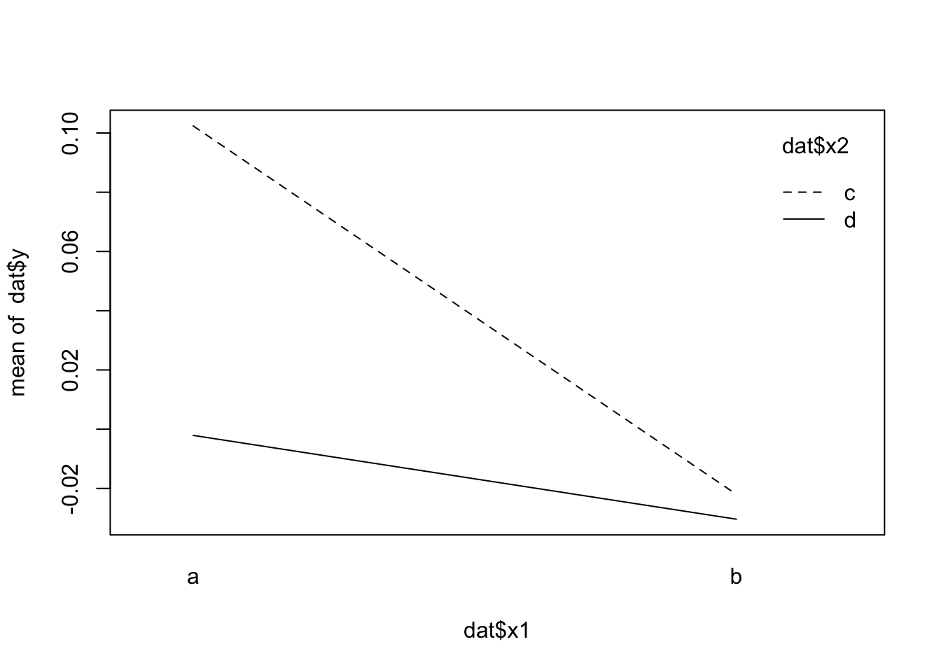
# plot
interaction.plot(dat$x1, dat$x2, dat$y, fun = mean)
# interaction x1:x2

int <- aggregate(y ~ x1 + x2, data = dat, mean)
int <- tidyr::pivot_wider(int, names_from = c(x1, x2), values_from = y)
intx1x2 <- (int$a_c - int$a_d) - (int$b_c  - int$b_d)

# model

fit <- lm(y ~ x1 * x2, data = dat)

car::Anova(fit, type = "3")
Anova Table (Type III tests)

Response: y
            Sum Sq Df F value Pr(>F)
(Intercept)  0.011  1  0.0119 0.9134
x1           0.117  1  0.1207 0.7292
x2           0.064  1  0.0660 0.7980
x1:x2        0.046  1  0.0478 0.8275
Residuals   73.364 76
rbind("model" = coef(fit),
      "manual" = c(gm, mx1, mx2, intx1x2))
       (Intercept)         x11         x21    x11:x21
model   0.01197932 -0.07633766 -0.05642767 0.09607497
manual  0.01197932 -0.07633766 -0.05642767 0.09607497