x1 <- c("a", "b")
x2 <- c("c", "d")

dat <- expand.grid(id = 1:20, x1 = x1, x2 = x2)
contrasts(dat$x1) <- c(-0.5, 0.5)
contrasts(dat$x2) <- c(-0.5, 0.5)
dat$y <- rnorm(nrow(dat))

# grand mean (intercept)

gm <- mean(aggregate(y ~ x1 + x2, data = dat, mean)$y)

# main effect x1

mx1 <- diff(aggregate(y ~ x1, data = dat, mean)$y)

# main effect x2

mx2 <- diff(aggregate(y ~ x2, data = dat, mean)$y)

# plot

interaction.plot(dat$x1, dat$x2, dat$y, fun = mean)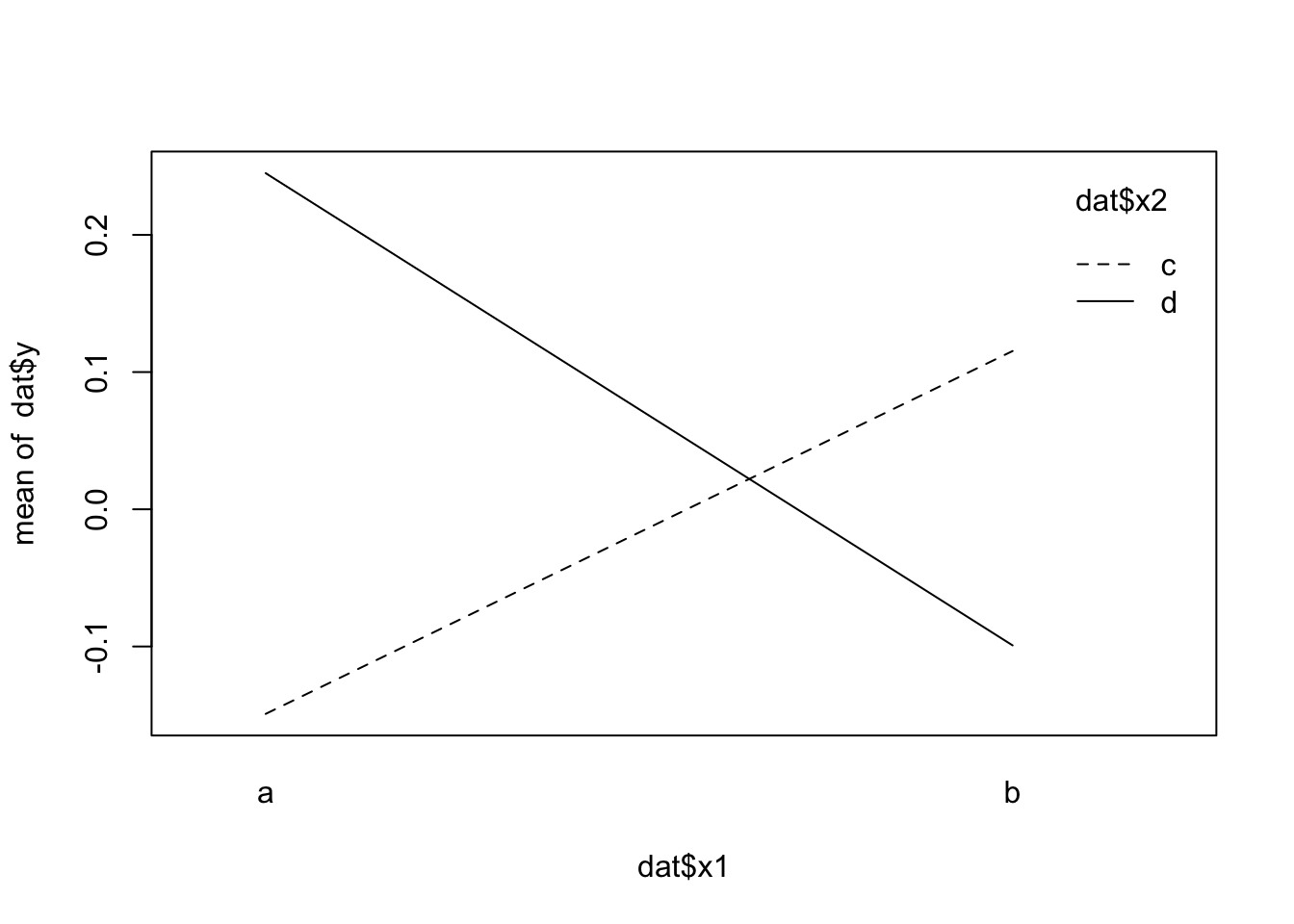
# interaction x1:x2

int <- aggregate(y ~ x1 + x2, data = dat, mean)
int <- tidyr::pivot_wider(int, names_from = c(x1, x2), values_from = y)
intx1x2 <- (int$a_c - int$a_d) - (int$b_c  - int$b_d)

# model

fit <- lm(y ~ x1 * x2, data = dat)

car::Anova(fit, type = "3")
Anova Table (Type III tests)
Response: y
Sum Sq Df F value Pr(>F)
(Intercept) 0.063 1 0.0575 0.8111
x1 0.032 1 0.0291 0.8649
x2 0.161 1 0.1479 0.7016
x1:x2 1.852 1 1.6990 0.1964
Residuals 82.834 76 rbind("model" = coef(fit),
"manual" = c(gm, mx1, mx2, intx1x2)) (Intercept) x11 x21 x11:x21
model 0.0279989 -0.03985257 0.08977371 -0.6085673
manual 0.0279989 -0.03985257 0.08977371 -0.6085673