3 Probability of Replication
Y
Key Readings
Key readings:
- Miller (2009) What is the probability of replicating a statistically significant effect?
- Pawel & Held (2020) Probabilistic forecasting of replication studies
Optional readings:
3.1 Formalization
3.1.1 The Miller (2009) definitions
Miller (2009) proposed one of the earliest probabilistic frameworks for estimating the probability of replication. He defines two different senses of replication probabilities:
aggregate replication probability (ARP): the probability of researchers working on a certain research field finding a statistically significant result in a replication study given a significant original study.
individual replication probability (IRP): the probability of finding a significant effect on a replication study when replicating a specific original study.
In this chapter we will take inspiration from Miller’s definitions and provide a formal framework to answer key questions about replication probabilities.
- What is the probability of replicating an observed effect in a precise replication experiment?
- What is the probability of replicating experiments of a certain type within a research field?
- How is the probability of replication affected by the experimental design (e.g., sample size, etc.) and by the effect size?
- Is the probability of replication affected by questionable research practices or publication bias?
3.1.2 Notation
We begin by providing a consistent notation and terminology, and a formal framework for the statistical models and analysis examples throughout the book. The notation is based on the replication model by Pawel & Held (2020) and the meta-analytical notation by Hedges & Schauer (2021), Schauer & Hedges (2021), and Hedges & Schauer (2019).
We use \(x\)’s to denote predictors, treatments, and fixed factors, and \(y\)’s to denote outcomes. The subscript \(i\) denotes individuals within a study, while \(r\) indexes studies. We use \(r=0\) to denote the original study, and \(r = 1, 2, \ldots, R\) to denote the \(R \geq 1\) replication studies.
We use the greek letter \(\theta\)’s to define the true effects for the original and replication study(s). These are population parameters. In particular \(\theta_0\) is the effect in original study and \(\theta_r\) is the effect in the \(r\)-th study. In principle, \(\theta\)’s can be vector valued, but for simplicity we will focus on a scalar effect. We will also use other greek letters for parameters specific to individual settings.
The one-to-one replication design is used when a single replication study is replicating an original experiment. On the other hand, a replication project with \(R\) replication studies is called a one-to-many design.
In Chapter 1 we covered the Machery definition of replication, in which only the randomly drawn subjects differ between the original study and the replications. In a replication of this type, the population of reference remains the same, an therefore \(\theta_0 = \theta_1 = \ldots = \theta_R\). This will be the case with Miller’s original models, for example. Generally, in a highly precise replication, this will also be approximately correct.
On the other hand, if we consider a group of extension experiments, or even more broadly examine an entire field of research, we typically alter fixed factors, and thus consider many different, albeit related, populations. In this case, the \(\theta\)’s will no longer be identical. Variation between \(\theta\)’s is an important aspect of replicability analysis. We will return to it in several places. For now, keep in mind that this variation depends on the unverse of studies of interest. For example, a group of extension experiments for a specific treatment / outcome combination will generally have smaller variability than a collection of experiments considering the effect of the same treatment on a variety of outcomes.
3.1.3 Two-Level Models
One way to think about studying the variation of the \(\theta\)’s is to frame the analysis in a two-level model. Within a study, we imagine that subjects are drawn from a population, with each population associated with a specific study design / fixed factors. In turn, then, study designs themselves are seen as draws from a hypothetically vast collection of possible designs. This allows to describe the variation of \(\theta\)’s probabilistically. In many examples we will use a Normal distribution to describe the resulting population of effect sizes. This normal distribution will have mean \(\mu_{\theta}\) and variance \(\tau^2\).
Replication is often framed in terms of tests of hypothesis. Parenthetically, several fields of study are making organized attempts at moving scientific reporting away from tests of hypotheses (Harrington et al., 2019). Evidential summaries from hypothesis tests, such as p-values, systematically confound sample size and effect size (Wasserstein & Lazar, 2016). Better reporting focuses on quantitative effect sizes. Nonetheless, replicability analysis requires explicit consideration of significance, as this remains a factor in determining publication.
Here we will define the null hypothesis to be that “the effect is too small to be of scientific interest”. Formally, the null hypothesis is true when \(|\theta| < h_0\) where \(h_0\) is specified by the analyst and defines a so-called region of practical equivalence or ROPE (Kruschke, 2015; Kruschke & Liddell, 2018)1. In a precise replication, \(\theta\) does not change across studies and thus the truth-value of the null hypothesis is invariant across studies. In contrast, if we consider a group of extension experiments or a whole field, the \(\theta\)’s vary and the null hypothesis may hold in some studies and not others. We will use \(\pi\) to denote the proportion of non-null effect in a population of studies.
Miller (2009) notes that \(\pi\) is an unknown quantity which is difficult to estimate from the literature. In Psychology, Wilson & Wixted (2018) tried to estimate \(\pi\) based on the Collaboration & Open Science Collaboration (2015) large scale replication project, which found different rates for social and cognitive psychology. In a similar vein, Jager & Leek (2014) tried to estimate the false discovery rate across the top medical journals.
The more precise the replication, the smaller the value of \(\tau\) will be. As \(\tau\) goes to zero, all \(\theta\)’s will concentrate around \(\mu_{\theta}\) and \(\pi\) will approach either 0 or 1 depending on whether \(\mu_{\theta}\) is in the region of practical equivalence.
Figure 3.1 depicts this simple generative model. The idea is that true effects in a given research area \(\theta_r\) come from a normal distribution with mean \(\mu_\theta\) and standard deviation \(\tau\). Within this research area, we have a certain proportion of true \(\pi\) and false \(1 - \pi\) effects. In the case of false effects, we can imagine a ROPE in which the effects are assumed to be equal to zero. Then the true effects \(\theta_r\) can be the target of an original study \(\hat \theta_0\) and one or more replication studies \(\hat \theta_r\) (\(r = (1, \ldots, R)\)). If the study is a precise replication, the heterogeneity is expected to be close to zero while in an extension experiment, we expect to see more heterogeneity. To simplify, the expected heterogeneity of a very precise replication is zero and all studies are essentially estimating the same original true effect \(\theta_0\). In cases where the heterogeneity is different from zero (i.e., an extension) each replication study is associated with a different underlying true effect \(\theta_r\). The degree of heterogeneity is related to the degree of precision, viz., to the number and relevance of changes to fixed factors. This model is similar to a random-effects meta-analysis (described in Chapter 4). The model can also be used to simulate replication studies as will be shown in ?sec-planning.

3.1.4 Multi-level Model
Figure 3.1 provides an example of a generating model for a specific research area in the literature, e.g., the distribution of true effects related to psychological treatments for depression. Some treatments in some conditions will have a higher/lower effect and in other conditions they will have a null effect. Extending the same reasoning to multiple effects within a broader literature, we can include another hierarchical layer in the model. Figure 3.2 depicts this extended model. For instance, we may be considering treatments for depression and anxiety. These research areas have specific average effects \(\mu_\theta^1, \mu_\theta^2\), heterogeneity \(\tau^1, \tau^2\) and proportions of true \(\pi^1, \pi^2\) and false \(1 - \pi^2, 1 - \pi^2\) effects. The combinatons of the two research areas define a broader literature, modeled as a mixture of these two distributions. Each component (i.e., anxiety and depression distributions) is associated with a weight \(\omega^1, \omega^2\), representing the importance (e.g., prevalence of studies) in the final mixture distribution. Finally, instead of considering \(\mu_\theta\) and \(\tau\) as fixed, we can sample these values from two distributions generating a more realistic research area contanining a larger set of true effects. In terms of replication, we can apply the same logic of Figure 3.1 where the degree of precision determines the expected heterogeneity in the replication/extension study.

3.1.5 Simple Null Hypotheses
Miller (2009) and many other works in the literature are concerned with simple null hypotheses. In our notation the null hypothesis is true when \(|\theta| = 0\). The logic of section Section 3.1.3 can be adapted to this case, as illustrated in Figure Figure 3.3. Now the distribution of \(\theta\) has two components: a continuous component describing the variation of the effect assuming the effect is not zero, and a discrete component at exactly zero. The probability of drawing a nonzero effect will again be \(\pi\), which is also the area under the bell curve in the figure. Thus the point mass at zero is \(1-\pi\). In terms of replication, we can apply the same logic of Figure 3.1 and Figure 3.2 where the degree of precision determines the expected heterogeneity in the replication/extension study.

3.2 Probability of Replication in Exact Replication Experiments
3.2.1 Two-Sample Design Review
We will often use a two-sample design to make the discussion more concrete. Assuming the homogeneity of variances among the two groups, the \(t\) statistic is calculated as follows:
\[ t = \frac{\overline{y}_1 - \overline{y}_2}{SE_{\overline{y}_1 - \overline{y}_2}} \tag{3.1}\]
where subscripts denote the two groups. The standard error in the denominator is: \[ \mbox{SE}_{\overline{y}_1 - \overline{y}_2} = s_p \sqrt{\frac{1}{n_1} + \frac{1}{n_2}} \tag{3.2}\]
where \(s_p\) is the pooled standard deviation: \[ s_p = \sqrt{\frac{s^2_{y_1}(n_1 - 1) + s^2_{y_1}{(n_2 - 1)}}{n_1 + n_2 - 2}} \tag{3.3}\]
In the case of a simple null hypothesis, the p-value can be calculated from a \(t\) distribution with \(\nu = n_1 + n_2 - 2\) degrees of freedom.
More generally, when the true effect size is not zero, the \(t\) statistic will follow a non-central Student’s \(t\) distribution with \(\nu\) degrees of freedom and non-centrality parameter \(\lambda\), calculated as follows: \[ \lambda = \delta \sqrt{\frac{n_1 n_2}{n_1 + n_2}} \tag{3.4}\]
where \(\delta\) is the true effect size — the true difference between means divided by the true group specific standard error.
If \(F_{t_\nu}\) is the cumulative distribution function of the non-central Student’s \(t\) distribution, the statistical power is calculated as:
\[ 1 - \beta = 1 - F_{t_\nu} \left(t_c, \lambda \right) + F_{t_\nu} \left(-t_{c}, \lambda \right) \tag{3.5}\]
With this setup, we can easily implement these equations in R, thus creating a flexible set of functions to reproduce and extend the examples from Miller (2009).
power.t(d = 0.5, n1 = 30)
## [1] 0.4778965
power.t(d = 0.5, n1 = 100)
## [1] 0.9404272
power.t(d = 0.1, n1 = 200)
## [1] 0.1694809
When the null hypothesis is a set (section Section 3.1.3) the p-value is calculated conditional on the least favorable case, which occurs when \(\theta = h_0\) or \(\theta = - h_0\), so the noncentral \(t\) is used to compute both the p-value and the power.
Another possibility is to use the full ROPE for the statistical test within the so-called equivalence testing framework (Lakens et al., 2018; see also Goeman et al., 2010 for the three-sided hypothesis testing).
3.2.2 The Calculus of Replication Probabilities
Consider the case of strict replication, so the null hypothesis has the same truth-value in both studies.
To prepare for Miller (2009), we look at replication probability by focusing on replicating significance. Given that the original study was significant (that is that \(|t_0| > t_{c_0}\)), what is the probability that the second study will also be significant and the effect will be in the same direction as the original study? Formally we express significance in the original study as \(|t_0| > t_{c_0}\), significance in the replication study as \(|t_1| > t_{c_1}\), and concordance of the direction of the effect as \(t_0 \cdot t_1 > 0\).
\[ p_{rep} = \Pr(|t_1| > t_{c_1} \cap t_0 \cdot t_1 >0 \boldsymbol{\mid} |t_0| > t_{c_0}) \tag{3.6}\]
Using the laws of conditional and total probability in turn, We can express this as
\[ \begin{split} p_{rep} &= \Pr(|t_1| \geq t_{c_1} \boldsymbol{\mid} |t_0| \geq t_{c_0}) \\[10pt] &= \frac{\Pr(|t_1| \geq t_{c_1} \cap t_0 \cdot t_1 >0 \cap |t_0| \geq t_{c_0})}{\Pr(|t_0| \geq t_{c_0})} \\[10pt] \end{split} \tag{3.7}\]
Considerering separately the numerator and the denominator, and using the law of total probability, we have:
\[ \begin{split} \mbox{numerator} =& \Pr(H_1) \cdot \Pr(|t_1| \geq t_{c1} \cap t_0 \cdot t_1 >0 \cap |t_0| \geq t_{c_0} \mid H_1) + \\ & \Pr(H_0) \cdot \Pr(|t_1| \geq t_{c1} \cap t_0 \cdot t_1 >0 \cap |t_0| \geq t_{c0} \mid H_0) \\[10pt] \mbox{denominator} =& \Pr(H_1) \cdot \Pr(|t_0| \geq t_{c_0} \mid H_1) + \\ & \Pr(H_0) \cdot \Pr(|t_0| \geq t_{c_1} \mid H_0). \end{split} \tag{3.8}\]
These expressions are a bit cumbersome, but they allow us to express the probability of replication as a useful function of power and significance level.
\[ \Pr (|t_0| \geq t_{c_0} | H_0 ) = \alpha_0, \quad \mbox{and} \quad \Pr (|t_0| \geq t_{c_0} \cap t_0 \cdot t_1 >0 | H_0 ) = \alpha_1 / 2 \tag{3.9}\]
where \(\alpha_r\) is the the study-specific significance level. The division by two is because half of the false positive rejections are expected to occur in the discordant direction under the null. Also
\[ \Pr(|t_0| \geq t_{c_0} | H_1) = 1-\beta_0 \quad \mbox{and} \quad \Pr(|t_1| \geq t_{c_1} \cap t_0 \cdot t_1 >0 | H_1) \approx 1-\beta_1 \tag{3.10}\]
where \(1-\beta_r\) is the study specific power. Power is simple to compute when the alternative is also a single point, but it is more complex when, as in section Section 3.1.3, we consider a distribution of non-null effects. For now, think about \(1-\beta_r\) as an average power. We will return on this point when we discuss hierarchical models.
The approximation sign \(\approx\) refers to the fact that we are ignoring the probability that the replication study will generate a significant and discordant effect if the true effect is not null and is indeed in the direction identified in the original study. This probability will be small when the sample size is large or the effect size is large, but can be nontrivial in small studies with small effects.
Rewriting and using independence of the two studies:
\[ \begin{split} p_{rep} & \approx \frac{\Pr(H_1) \cdot (1-\beta_0)(1-\beta_1) + (1- \Pr(H_1)) \cdot \alpha_0 \alpha_1 / 2}{\Pr(H_1) \cdot (1-\beta_0) + (1-\Pr(H_1)) \cdot \alpha_0} \\[10pt] \end{split} \tag{3.11}\]
The key quantity that remains to be explained is \(\Pr(H_1)\), the probability that the effect is not null. The interpretation of this probability depends on the context as well as the analysts’ approach. In section Section 3.2.3 we consider Miller’s version, where \(\Pr(H_1)\) is essentially \(\pi\) from Section Section 3.1.3. Later on, we will discuss an alternative Bayesian interpretation, where \(\Pr(H_1)\) is based on expert knowledge existing prior to the original experiment.
We take two quick digressions before going back to Miller. First, if \(R>1\) we can extend this reasoning to more general expressions. For example if we want to estimate the probability of having successful replications in \(R\) experiments we can consider \[ \Pr \left( \bigcap_{r=1}^R |t_r| > t_{c_r} \boldsymbol{\mid} |t_0| > t_{c_0} \right). \tag{3.12}\]
Second, if you are not familiar with the logic behind Bayes’s rule, we will walk you through it in the remainder of this section. The probability of the event A happening given (\(|\)) that B happened is:
\[ \Pr(A|B) = \frac{\Pr(A \cap B)}{\Pr(B)} \tag{3.13}\]
Where \(\Pr(A \cap B)\) is the joint probability that can be calculated as:
\[ \Pr(A \cap B) = \Pr(B|A) \cdot \Pr(A) \tag{3.14}\]
Then the full equation also known as Bayes rule is:
\[ \Pr(A|B) = \frac{\Pr(B|A) \cdot \Pr(A)}{\Pr(B)} \tag{3.15}\]
3.2.3 Miller’s Aggregate Replication Probability (ARP)
To recap, Miller (2009) is about replication with the highest precision, because he considers no differences in populations between the experiments. He focuses on tests of hypotheses, and considers replication of experiments with significant testing results, as we did above. He also assumes that power and significance level are the same in the original and replication experiment. And, he evaluates power at a single point at a time, effectively assuming that the statistical problem is testing a simple null hypothesis against a simple alternative.
With regards to \(\Pr( H_1)\) he considers a scheme similar to that of section Section 3.1.3. A study design is drawn randomly from the aggregate describing a scientific field of interest, and then replicated with high precision. In what proportion of cases does this exercise lead to a replication? For this calculation \(\Pr( H_1)\) is the same as \(\pi\) in Figure 3.1. Miller calls \(\pi\) the strength of a research area. This parameter has also been considered by other authors when evaluating the probability of replication within a research field (Ioannidis, 2005; Wilson & Wixted, 2018).
In Miller’s setting, the only relevant parameters in the replication model are the type-2 error rate \(\beta\) (or equivalently the statistical power \(1 - \beta\)), the type-1 error rate \(\alpha\) and the proportion of true hypotheses \(\pi\) in a certain research field.
Using formula Equation 3.11, the probability of replicating an effect in a given research area (ARP), conditional on a significant original experiment, is \[ p_{ARP} \approx \frac {\pi \cdot (1 - \beta)^2 + (1 - \pi) \cdot \alpha^2 / 2} {\pi \cdot (1 - \beta) + (1 - \pi) \cdot \alpha} \tag{3.16}\]
The denominator is the probability of a significant result in the original study, broken down into the probability of a false positive \((1 - \pi) \alpha\) plus the probability of a true positive \(\pi (1 - \beta)\). Now, let’s consider the numerator. This is the probability that both the original and replication studies are significant and also concordant in the sign of their effects.
A good way to understand the process is by formalizing inference using a contingency table as done in Table 3.1.
| False | True | |||
|---|---|---|---|---|
| \(\boldsymbol{H_0}\) | False | True Positive (\(1 - \beta\)) | False Negative (\(\beta\)) | \(\pi\) |
| \(\boldsymbol{H_0}\) | True | False Positive (\(\alpha\)) | True Negative (\(1 - \alpha\)) | \(1 - \pi\) |
For example, the probability that something is significant is the sum of true positives (i.e., the statistical power) and false positives (i.e., type-1 errors) weighted by the prevalence \(\pi\). Thus the numerator \(\Pr(|t_1| > t_{c1} \cap |t_0| > t_{c0})\) can be written as the sum of the following two quantities:
- Original study being significant \((1 - \beta) \cdot \pi + \alpha \cdot (1 - \pi)\)
- Replication study being significant \((1 - \beta) + \frac{\alpha}{2}\)
We have \(\frac{\alpha}{2}\) in the second expression because we assume that replication success happens when the effect is in the same direction, i.e., we are ignoring false positives with opposite sign.
An interesting use of Equation 3.11 and Equation 3.16 is that we can explore the probability of replication in different scenarios by manipulating the parameters defined above. Ulrich & Miller (2020) improved and extended Miller (2009), by estimating the impact of questionable research practices on the probability of replication. They found that the most important parameter negatively impacting replication rates is \(\pi\), with questionable research practices having only a minor impact.
3.2.4 R Code for the Aggregate replication probability (ARP)
We implemented the Miller (2009) equations in R (see also ?arp):
arp <- function(R, pi, power, alpha) {

    if(any(R < 2)) stop("number of studies should be equal or greater than 2")

    if(length(power) != 1 & length(power) != R){
      stop("length of power vector should be 1 or R")
    }

    if(length(power) == 1) power <- rep(power, R)

    num <- pi * prod(power) + (1 - pi) * alpha * (alpha/2)^(R - 1)
    den <- pi * power[1] + (1 - pi) * alpha
    num/den
}
r is the number of replication studies, pi is \(\pi\), power is \(1 - \beta\) and alpha is \(\alpha\).
The Figure 3.4 depicts how the ARP changes as we vary the theory strength \(\pi\) and the power (assumed to be the same for the original and replication experiment).
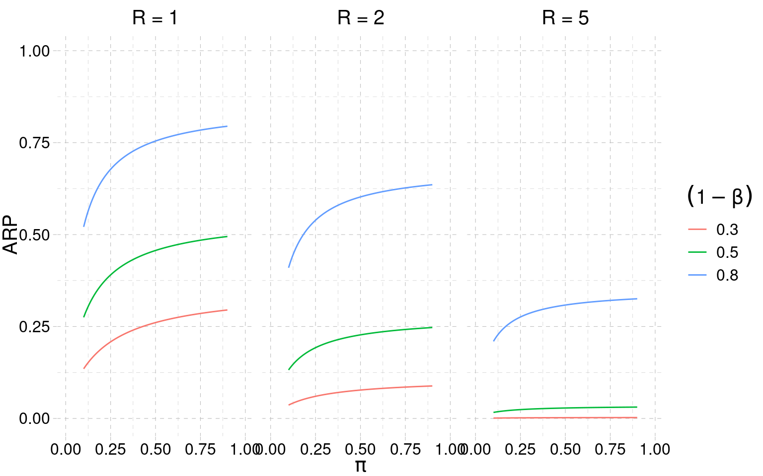
The main takeaways from Figure 3.4 are:
- for medium (and probably plausible) levels of theory strength \(\pi\), the replication probabilities are relatively low — even when the power is high
- when \(R > 1\), the replication probabilities are very low — in all conditions
3.2.5 Miller’s Individual replication probability (IRP)
In contrast to the ARP, which considers a randomly drawn original study from a field, the individual replication probability (IRP) focuses on a specific original study. Miller’s approach is ask what is the probability of a significant and concordant test result in the replication study, supposing that the estimated effect in the original study is correct. This reduces to calculating the power of the replication study, conditional upon the observed effect, that is: \(p_{IRP} = 1 - \beta(\hat\theta_0)\)
Using the Equations from Section 3.2.1, we can reproduce and extend the Miller (2009) figures. Basically, we estimate the IRP assuming that the power (thus the effect size and sample size) of the replication study is the same as that of the original study. The key function is p2d, which returns the power, given the effect size, for the point estimate; and, the lower/upper limit of the effect size confidence interval2.
p2d <- function(p, n, alpha = 0.05){
    df <- n*2 - 2
    to <- abs(qt(p/2, df))
    se <- sqrt(1/n + 1/n)
    cit <- effectsize:::.get_ncp_t(to, df)
    lb.t <- cit[1]
    ub.t <- cit[2]
    d <- to * se
    lb <- lb.t * se
    ub <- ub.t * se
    # power
    d.power <- power.t(d = d, n1 = n, alpha = alpha)
    lb.power <- power.t(d = lb, n1 = n, alpha = alpha)
    ub.power <- power.t(d = ub, n1 = n, alpha = alpha)
    list(t = to, d = d,
         se = se, df = df,
         ci.lb = lb, ci.ub = ub,
         d.power = d.power,
         lb.power = lb.power,
         ub.power = ub.power,
         p = p)
}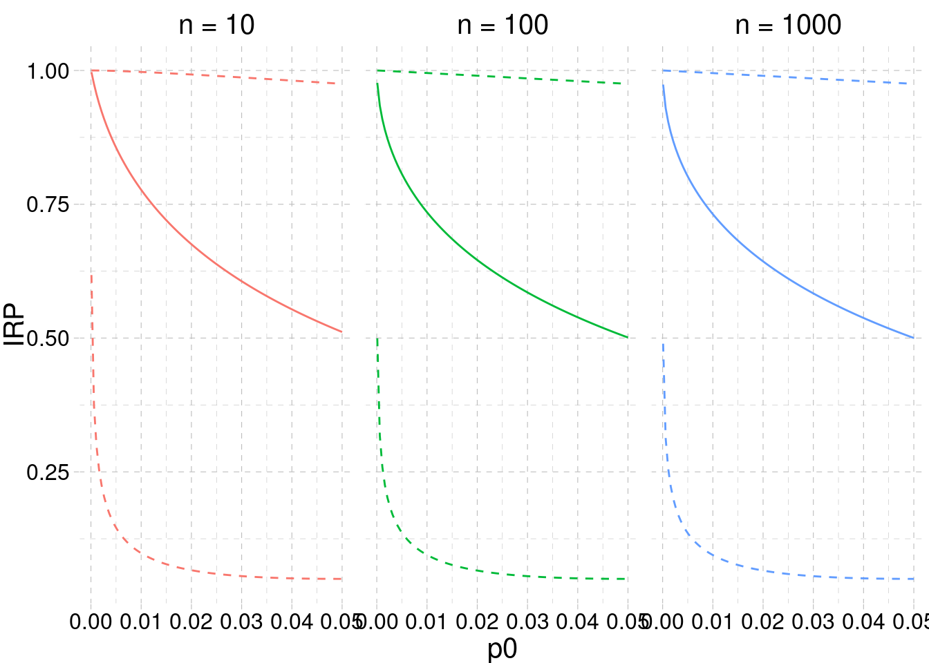
The most important takeaway from Figure 3.5 is that the statistical significance of the original experiment alone \(p_0 \leq \alpha\) is not enough to reliably estimate the probability of replicating the effect. Only when the p-value is very small is the range of expected power relatively narrow. For significant but higher p-values there is a lot of uncertainty vis-á-vis the IRP. In this context, Perugini et al. (2014) have recommended against the use of the point estimate of an effect size to plan a new study (e.g., a replication). A more conservative approach would be to use another value (e.g., the lower bound) of the \((1 - \alpha) \cdot 100\) confidence interval. This conservative approach can mitigate the likely overestimation of the original study, thus providing a more realistic estimation of the probability of replication.
3.2.6 Bayesian Individual Replication Probability
Miller’s IRP has two main limitations. First, the effect size estimated in the original study is subject to sampling variability. This is not considered by Miller. In reality, the effect size could be larger or smaller. Second, in scientific areas where finding large effects is more challenging, the true effect size is more likely to be smaller, relative to those estimated for research areas in which large effects abound. So, considering a study in isolation is a limitation. Even at the individual level, we should expect a higher probability of replication for research areas where there are more true effects to be found. Some of these limitations can be mitigated by Bayesian replication probabilities. If you are not familiar with the logic behind Bayesian statistics, Lindley (1972) provides an excellent introduction.
For a simple example, consider specifying \(\Pr(H_1)\) for the individual experiment at hand to reflect knowledge exisitng up to the point of the original experiment, but not including the original experiment itself. In the depression treatment example, this may have to to with the strength of the hypothesis, the plausibility of treatment examined, prior experiments in animals if the original experiment is in humans etc. Then one can apply the calculus of Section Section 3.2.2 (and specifically Equation 3.16) to evaluate the individual replication probability. Consideration of the sampling variability in the effect size may be incorporated in the specific way one calculates the average power. Consideration of the strength of the field of study can be embedded in the prior, either informally or through the use of hierarchical models, which we discuss below.
3.3 Selection and Regression to the Mean
The original effect size estimation could be biased (usually inflated) for several reasons (e.g., publication bias) affecting the actual probability of replication. For example, let’s assume that original studies are published only when they are significant. In addition, let’s assume we are considering a research area with medium strength and with average medium-small effect sizes (a very likely scenario). Finally, let’s assume we are working with sample sizes that are relatively low. Such a research area will tend to be low-powered; and, significant effects will either be inflated (in the best case) or false positives (in the worst case).
When conducting replication studies of these kinds of original studies, we may find significant but substantially smaller estimated effects (or even non significant effects.) For example, the large scale project Collaboration & Open Science Collaboration (2015) reported that — regardless of significance level — replicated effects were substantially smaller than original effects. Regression to the mean is a good explanation of this phenomenon, since selection of extreme results will produce on average lower estimations (i.e., shrinkage) in later studies. In addition, if the replication study design (i.e., sample size) is based on the original effect size estimation, the inflation can greatly reduce the power. This is related to the concept of the type-M (M for magnitude) error (Gelman & Carlin, 2014), which quantifies the exent of inflation given the true effect and the sample size.
In Code 3.1, there is a small simulation showing how to estimate the type-M error for a two-sample design.
[1] 1.738048The type-M error increases as the sample size and/or the true effect size decreases. The Figure 3.6 shows the type-M error for different conditions.
Code
typeM <- function(d, n, B = 1e3){
    di <- pi <- rep(NA, B)
    for(i in 1:nsim){
        g0 <- rnorm(n, 0, 1)
        g1 <- rnorm(n, d, 1)
        tt <- t.test(g1, g0)
        di[i] <- tt$statistic * tt$stderr
        pi[i] <- tt$p.value
    }
    significant <- pi <= 0.05
    mean(abs(di[significant])) / d
}

sim <- expand.grid(
    n = seq(10, 100, 10),
    d = c(0.1, 0.3, 0.5, 1),
    M = NA
)


for(i in 1:nrow(sim)){
    sim$M[i] <- typeM(sim$d[i], sim$n[i])
}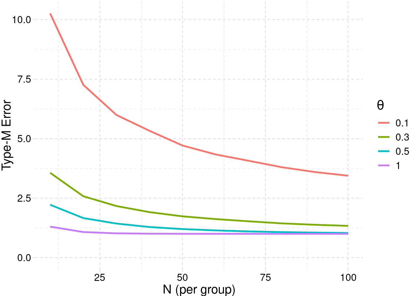
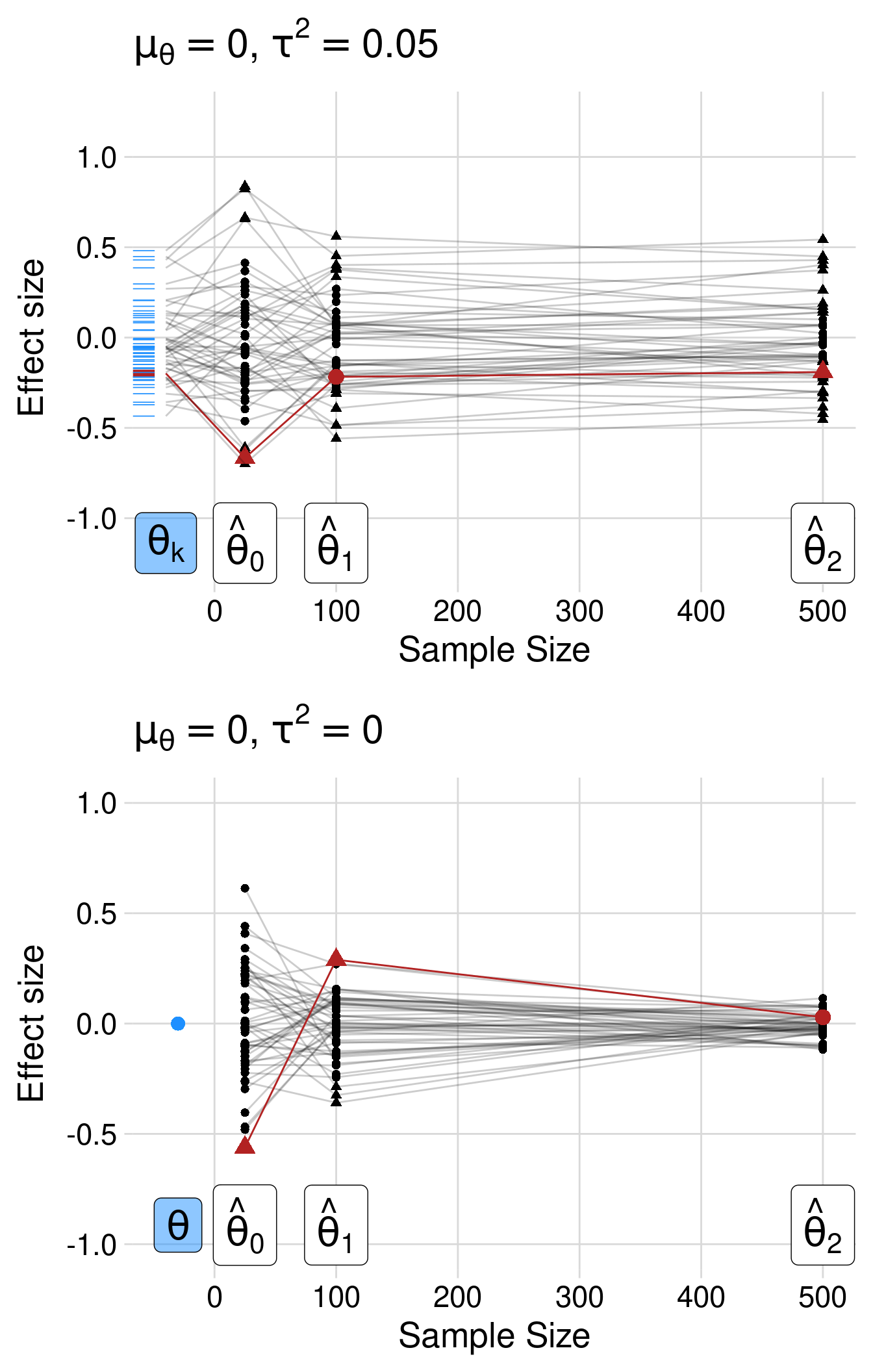
Figure 3.7 shows the impact of regression to the mean. We simulated two scenarios with a selection for extreme (i.e., significant) values, where the true average effect is zero. In the top panel, we included some heterogeneity — there is a distribution of true effects where the average size is zero. The selection occurs in a hypothetical original study with a sample size of 25. Then, we simulated two other studies with sample sizes 100 and 500, respectively, sampling from the same distribution and with the same true effect. The crucial lesson of Figure 3.7 is that selection of extreme studies will result in replication studies with lower power and smaller estimated effects. This is especially true if the replication study is based on the estimated effect of the original, low-powered study.
3.4 Probability of Replication in Extension Experiments
3.4.1 Hierarchical Models
Pawel & Held (2020) generalize the methodology of Miller (2009). Miller’s model neglected the possibility of heterogeneity among true effects, assuming that the power (and thus the effect size) is the same when \(H_0\) is false. A more sophisticated way to predict the probability of estimating a certain finding is to use the information of the original study and replication study (one-to-one replication) within a hierarchical bayesian model. Here are two main features of this more general modelling approach:
includes the uncertainty of both studies and eventually the between-study heterogeneity \(\tau\). This allows the replication study to be truly different from the original study (e.g., it allows us to take the effects of publication bias into account).
includes a shrinkage factor, balancing the strength of the original study and the between-study heterogeneity, which allows us to account for regression to the mean and effect size inflation of the original study.
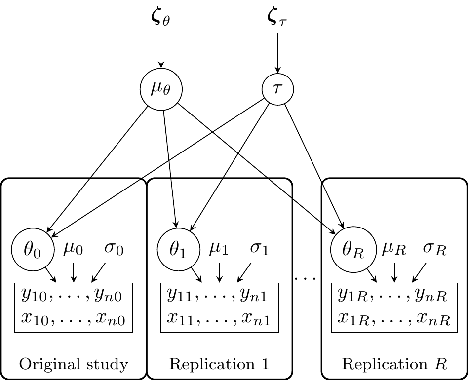
We adapted the Pawel & Held (2020) model, creating a more general version that can be easily adapted to simulating and analyzing data from replication studies as well as predicting the probability of replication given the model parameters. The generalized version of the model is presented in Figure 3.8. (The actual model will be implemented in Chapter 4.)
In the simple case of a two-group study, where \(x_{ir}\) denotes whether individual \(i\) is in group one, the distribution of the data in study \(r\) is as follows:
\[ y_{ir}|x_{ir} \sim \mathcal{N}(\mu_r + x_{ir}\theta_r, \sigma_r) \]
In this case, \(\theta_r\) can be intepreted as the mean difference between the two groups.
At the effect size level, for example, we may have:
\[ \theta_r \sim \mathcal{N}(\mu_\theta, \tau) \]
Figure 3.8 depicts the hierarchical model. \(\mu_\theta\) is the average true effect and \(\tau\) is the heterogeneity thus the standard deviation of the true effects. This is very similar to the generating model presented in Figure 3.1 and can be considered as a standard two-level model (or a random-effects meta-analysis). Both \(\mu_\theta\) and \(\tau\) can be associated with a prior distribution. In this case \(\boldsymbol{\zeta_\theta}\) and \(\boldsymbol{\zeta_\tau}\) are vectors of parameters of the prior distributions. A common choice would be a normal distribution for \(\mu_\theta\) and an half-cauchy distribution for \(\tau\) (Williams et al., 2018). At the study level, \(\theta_r\) is the study-specific slope (i.e., the difference between the groups), \(\mu_t\) is the intercept (i.e., expected value for the reference group). \(y_{nr}\) and \(x_{nr}\) are the response values and the predictors (respectively) for the individual \(n\) of the study \(r\).
The model can be easily implemented in R using the probabilistic programming language STAN (Stan Development Team, 2021) or, under some conditions, using the analytical form as used in Pawel & Held (2020).
3.5 Key Questions
- How do questionable research practices and publication bias influence our expectations about replication?
- What is the difference between individual replication probability (IRP) and aggregate replication probability (ARP)?
- Is there a different scientific value in replications vs exensions?
References
To note that the term ROPE refer to the Bayesian version of the equivalence region in the frequentist equivalence testing approach (Lakens et al., 2018). Despite using the Bayesian term, we are just referring to an area where the effect is neglegible and equivalent to a point-null value (e.g, zero).↩︎
To calculate the confidence interval of the effect size we used the so-called pivot method (Steiger, 2004) implemented into the
effectsize:::.get_ncp_t()function↩︎